This Quantum World/Feynman route/From quantum to classical

From quantum to classical

Action

Let's go back to the propagator

$\langle B|A\rangle =\int \!{\mathcal {DC}}\,Z[{\mathcal {C}}:A\rightarrow B].$

For a free and stable particle we found that

$Z[{\mathcal {C}}]=e^{-(i/\hbar )\,m\,c^{2}\,s[{\mathcal {C}}]},\qquad s[{\mathcal {C}}]=\int _{\mathcal {C}}ds,$

where $ds={\sqrt {dt^{2}-(dx^{2}+dy^{2}+dz^{2})/c^{2}}}$ is the proper-time interval associated with the path element $d{\mathcal {C}}$. For the general case we found that the amplitude $Z(d{\mathcal {C}})$ is a function of $t,x,y,z$ and $dt,dx,dy,dz$ or, equivalently, of the coordinates $t,x,y,z$, the components $c\,dt/ds,dx/ds,dy/ds,dz/ds$ of the 4-velocity, as well as $ds$. For a particle that is stable but not free, we obtain, by the same argument that led to the above amplitude,

$Z[{\mathcal {C}}]=e^{(i/\hbar )\,S[{\mathcal {C}}]},$

where we have introduced the functional $S[{\mathcal {C}}]=\int _{\mathcal {C}}dS$, which goes by the name action.

For a free and stable particle, $S[{\mathcal {C}}]$ is the proper time (or proper duration) $s[{\mathcal {C}}]=\int _{\mathcal {C}}ds$ multiplied by $-mc^{2}$, and the infinitesimal action $dS[d{\mathcal {C}}]$ is proportional to $ds$:

$S[{\mathcal {C}}]=-m\,c^{2}\,s[{\mathcal {C}}],\qquad dS[d{\mathcal {C}}]=-m\,c^{2}\,ds.$

Let's recap. We know all about the motion of a stable particle if we know how to calculate the probability $p(B|A)$ (in all circumstances). We know this if we know the amplitude $\langle B|A\rangle$. We know the latter if we know the functional $Z[{\mathcal {C}}]$. And we know this functional if we know the infinitesimal action $dS(t,x,y,z,dt,dx,dy,dz)$ or $dS(t,\mathbf {r} ,dt,d\mathbf {r} )$ (in all circumstances).

What do we know about $dS$?

The multiplicativity of successive propagators implies the additivity of actions associated with neighboring infinitesimal path segments $d{\mathcal {C}}_{1}$ and $d{\mathcal {C}}_{2}$. In other words,

$e^{(i/\hbar )\,dS(d{\mathcal {C}}_{1}+d{\mathcal {C}}_{2})}=e^{(i/\hbar )\,dS(d{\mathcal {C}}_{2})}\,e^{(i/\hbar )\,dS(d{\mathcal {C}}_{1})}$

implies

$dS(d{\mathcal {C}}_{1}+d{\mathcal {C}}_{2})=dS(d{\mathcal {C}}_{1})+dS(d{\mathcal {C}}_{2}).$

It follows that the differential $dS$ is homogeneous (of degree 1) in the differentials $dt,d\mathbf {r}$:

$dS(t,\mathbf {r} ,\lambda \,dt,\lambda \,d\mathbf {r} )=\lambda \,dS(t,\mathbf {r} ,dt,d\mathbf {r} ).$

This property of $dS$ makes it possible to think of the action $S[{\mathcal {C}}]$ as a (particle-specific) length associated with ${\mathcal {C}}$, and of $dS$ as defining a (particle-specific) spacetime geometry. By substituting $1/dt$ for $\lambda$ we get:

$dS(t,\mathbf {r} ,\mathbf {v} )={\frac {dS}{dt}}.$

Something is wrong, isn't it? Since the right-hand side is now a finite quantity, we shouldn't use the symbol $dS$ for the left-hand side. What we have actually found is that there is a function $L(t,\mathbf {r} ,\mathbf {v} )$, which goes by the name Lagrange function, such that $dS=L\,dt$.

Geodesic equations

Consider a spacetime path ${\mathcal {C}}$ from $A$ to $B.$ Let's change ("vary") it in such a way that every point $(t,\mathbf {r} )$ of ${\mathcal {C}}$ gets shifted by an infinitesimal amount to a corresponding point $(t+\delta t,\mathbf {r} +\delta \mathbf {r} ),$ except the end points, which are held fixed: $\delta t=0$ and $\delta \mathbf {r} =0$ at both $A$ and $B.$

If $t\rightarrow t+\delta t,$ then $dt=t_{2}-t_{1}\longrightarrow t_{2}+\delta t_{2}-(t_{1}+\delta t_{1})=(t_{2}-t_{1})+(\delta t_{2}-\delta t_{1})=dt+d\delta t.$

By the same token, $d\mathbf {r} \rightarrow d\mathbf {r} +d\delta \mathbf {r} .$

In general, the change ${\mathcal {C}}\rightarrow {\mathcal {C}}'$ will cause a corresponding change in the action: $S[{\mathcal {C}}]\rightarrow S[{\mathcal {C}}']\neq S[{\mathcal {C}}].$ If the action does not change (that is, if it is stationary at ${\mathcal {C}}$ ),

$\delta S=\int _{{\mathcal {C}}'}dS-\int _{\mathcal {C}}dS=0,$

then ${\mathcal {C}}$ is a geodesic of the geometry defined by $dS.$ (A function $f(x)$ is stationary at those values of $x$ at which its value does not change if $x$ changes infinitesimally. By the same token we call a functional $S[{\mathcal {C}}]$ stationary if its value does not change if ${\mathcal {C}}$ changes infinitesimally.)

To obtain a handier way to characterize geodesics, we begin by expanding

$dS({\mathcal {C}}')=dS(t+\delta t,\mathbf {r} +\delta \mathbf {r} ,dt+d\delta t,d\mathbf {r} +d\delta \mathbf {r} )$

$=dS(t,\mathbf {r} ,dt,d\mathbf {r} )+{\frac {\partial dS}{\partial t}}\,\delta t+{\frac {\partial dS}{\partial \mathbf {r} }}\cdot \delta \mathbf {r} +{\frac {\partial dS}{\partial dt}}\,d\delta t+{\frac {\partial dS}{\partial d\mathbf {r} }}\cdot d\delta \mathbf {r} .$

This gives us

$(^{*})\quad \int _{{\mathcal {C}}'}dS-\int _{\mathcal {C}}dS=\int _{\mathcal {C}}\left[{\partial dS \over \partial t}\delta t+{\partial dS \over \partial \mathbf {r} }\cdot \delta \mathbf {r} +{\partial dS \over \partial dt}d\,\delta t+{\partial dS \over \partial d\mathbf {r} }\cdot d\,\delta \mathbf {r} \right].$

Next we use the product rule for derivatives,

$d\left({\partial dS \over \partial dt}\delta t\right)=\left(d{\partial dS \over \partial dt}\right)\delta t+{\partial dS \over \partial dt}d\,\delta t,$

$d\left({\partial dS \over \partial d\mathbf {r} }\cdot \delta \mathbf {r} \right)=\left(d{\partial dS \over \partial d\mathbf {r} }\right)\cdot \delta \mathbf {r} +{\partial dS \over \partial d\mathbf {r} }\cdot d\,\delta \mathbf {r} ,$

to replace the last two terms of (*), which takes us to

$\delta S=\int \left[\left({\partial dS \over \partial t}-d{\partial dS \over \partial dt}\right)\delta t+\left({\partial dS \over \partial \mathbf {r} }-d{\partial dS \over \partial d\mathbf {r} }\right)\cdot \delta \mathbf {r} \right]+\int d\left({\partial dS \over \partial dt}\delta t+{\partial dS \over \partial d\mathbf {r} }\cdot \delta \mathbf {r} \right).$

The second integral vanishes because it is equal to the difference between the values of the expression in brackets at the end points $A$ and $B,$ where $\delta t=0$ and $\delta \mathbf {r} =0.$ If ${\mathcal {C}}$ is a geodesic, then the first integral vanishes, too. In fact, in this case $\delta S=0$ must hold for all possible (infinitesimal) variations $\delta t$ and $\delta \mathbf {r} ,$ whence it follows that the integrand of the first integral vanishes. The bottom line is that the geodesics defined by $dS$ satisfy the geodesic equations

${\partial dS \over \partial t}=d\,{\partial dS \over \partial dt},\qquad {\partial dS \over \partial \mathbf {r} }=d\,{\partial dS \over \partial d\mathbf {r} }.$

Principle of least action

If an object travels from $A$ to $B,$ it travels along all paths from $A$ to $B,$ in the same sense in which an electron goes through both slits. Then how is it that a big thing (such as a planet, a tennis ball, or a mosquito) appears to move along a single well-defined path?

There are at least two reasons. One of them is that the bigger an object is, the harder it is to satisfy the conditions stipulated by Rule $B.$ Another reason is that even if these conditions are satisfied, the likelihood of finding an object of mass $m$ where according to the laws of classical physics it should not be, decreases as $m$ increases.

To see this, we need to take account of the fact that it is strictly impossible to check whether an object that has travelled from $A$ to $B,$ has done so along a mathematically precise path ${\mathcal {C}}.$ Let us make the half realistic assumption that what we can check is whether an object has travelled from $A$ to $B$ within a a narrow bundle of paths — the paths contained in a narrow tube ${\mathcal {T}}.$ The probability of finding that it has, is the absolute square of the path integral $I({\mathcal {T}})=\int _{\mathcal {T}}{\mathcal {DC}}e^{(i/\hbar )S[{\mathcal {C}}]},$ which sums over the paths contained in ${\mathcal {T}}.$

Let us assume that there is exactly one path from $A$ to $B$ for which $S[{\mathcal {C}}]$ is stationary: its length does not change if we vary the path ever so slightly, no matter how. In other words, we assume that there is exactly one geodesic. Let's call it ${\mathcal {G}},$ and let's assume it lies in ${\mathcal {T}}.$

No matter how rapidly the phase $S[{\mathcal {C}}]/\hbar$ changes under variation of a generic path ${\mathcal {C}},$ it will be stationary at ${\mathcal {G}}.$ This means, loosely speaking, that a large number of paths near ${\mathcal {G}}$ contribute to $I({\mathcal {T}})$ with almost equal phases. As a consequence, the magnitude of the sum of the corresponding phase factors $e^{(i/\hbar )S[{\mathcal {C}}]}$ is large.

If $S[{\mathcal {C}}]/\hbar$ is not stationary at ${\mathcal {C}},$ all depends on how rapidly it changes under variation of ${\mathcal {C}}.$ If it changes sufficiently rapidly, the phases associated with paths near ${\mathcal {C}}$ are more or less equally distributed over the interval $[0,2\pi ],$ so that the corresponding phase factors add up to a complex number of comparatively small magnitude. In the limit $S[{\mathcal {C}}]/\hbar \rightarrow \infty ,$ the only significant contributions to $I({\mathcal {T}})$ come from paths in the infinitesimal neighborhood of ${\mathcal {G}}.$

We have assumed that ${\mathcal {G}}$ lies in ${\mathcal {T}}.$ If it does not, and if $S[{\mathcal {C}}]/\hbar$ changes sufficiently rapidly, the phases associated with paths near any path in ${\mathcal {T}}$ are more or less equally distributed over the interval $[0,2\pi ],$ so that in the limit $S[{\mathcal {C}}]/\hbar \rightarrow \infty$ there are no significant contributions to $I({\mathcal {T}}).$

For a free particle, as you will remember, $S[{\mathcal {C}}]=-m\,c^{2}\,s[{\mathcal {C}}].$ From this we gather that the likelihood of finding a freely moving object where according to the laws of classical physics it should not be, decreases as its mass increases. Since for sufficiently massive objects the contributions to the action due to influences on their motion are small compared to $|-m\,c^{2}\,s[{\mathcal {C}}]|,$ this is equally true of objects that are not moving freely.

What, then, are the laws of classical physics?

They are what the laws of quantum physics degenerate into in the limit $\hbar \rightarrow 0.$ In this limit, as you will gather from the above, the probability of finding that a particle has traveled within a tube (however narrow) containing a geodesic, is 1, and the probability of finding that a particle has traveled within a tube (however wide) not containing a geodesic, is 0. Thus we may state the laws of classical physics (for a single "point mass", to begin with) by saying that it follows a geodesic of the geometry defined by $dS.$

This is readily generalized. The propagator for a system with $n$ degrees of freedom — such as an $m$-particle system with $n=3m$ degrees of freedom — is

$\langle {\mathcal {P}}_{f},t_{f}|{\mathcal {P}}_{i},t_{i}\rangle =\int \!{\mathcal {DC}}\,e^{(i/\hbar )S[{\mathcal {C}}]},$

where ${\mathcal {P}}_{i}$ and ${\mathcal {P}}_{f}$ are the system's respective configurations at the initial time $t_{i}$ and the final time $t_{f},$ and the integral sums over all paths in the system's $n{+}1$-dimensional configuration spacetime leading from $({\mathcal {P}}_{i},t_{i})$ to $({\mathcal {P}}_{f},t_{f}).$ In this case, too, the corresponding classical system follows a geodesic of the geometry defined by the action differential $dS,$ which now depends on $n$ spatial coordinates, one time coordinate, and the corresponding $n{+}1$ differentials.

The statement that a classical system follows a geodesic of the geometry defined by its action, is often referred to as the principle of least action. A more appropriate name is principle of stationary action.

Energy and momentum

Observe that if $dS$ does not depend on $t$ (that is, $\partial dS/\partial t=0$ ) then

$E=-{\partial dS \over \partial dt}$

is constant along geodesics. (We'll discover the reason for the negative sign in a moment.)

Likewise, if $dS$ does not depend on $\mathbf {r}$ (that is, $\partial dS/\partial \mathbf {r} =0$ ) then

$\mathbf {p} ={\partial dS \over \partial d\mathbf {r} }$

is constant along geodesics.

$E$ tells us how much the projection $dt$ of a segment $d{\mathcal {C}}$ of a path ${\mathcal {C}}$ onto the time axis contributes to the action of ${\mathcal {C}}.$ $\mathbf {p}$ tells us how much the projection $d\mathbf {r}$ of $d{\mathcal {C}}$ onto space contributes to $S[{\mathcal {C}}].$ If $dS$ has no explicit time dependence, then equal intervals of the time axis make equal contributions to $S[{\mathcal {C}}],$ and if $dS$ has no explicit space dependence, then equal intervals of any spatial axis make equal contributions to $S[{\mathcal {C}}].$ In the former case, equal time intervals are physically equivalent: they represent equal durations. In the latter case, equal space intervals are physically equivalent: they represent equal distances.

If equal intervals of the time coordinate or equal intervals of a space coordinate are not physically equivalent, this is so for either of two reasons. The first is that non-inertial coordinates are used. For if inertial coordinates are used, then every freely moving point mass moves by equal intervals of the space coordinates in equal intervals of the time coordinate, which means that equal coordinate intervals are physically equivalent. The second is that whatever it is that is moving is not moving freely: something, no matter what, influences its motion, no matter how. This is because one way of incorporating effects on the motion of an object into the mathematical formalism of quantum physics, is to make inertial coordinate intervals physically inequivalent, by letting $dS$ depend on $t$ and/or $\mathbf {r} .$

Thus for a freely moving classical object, both $E$ and $\mathbf {p}$ are constant. Since the constancy of $E$ follows from the physical equivalence of equal intervals of coordinate time (a.k.a. the "homogeneity" of time), and since (classically) energy is defined as the quantity whose constancy is implied by the homogeneity of time, $E$ is the object's energy.

By the same token, since the constancy of $\mathbf {p}$ follows from the physical equivalence of equal intervals of any spatial coordinate axis (a.k.a. the "homogeneity" of space), and since (classically) momentum is defined as the quantity whose constancy is implied by the homogeneity of space, $\mathbf {p}$ is the object's momentum.

Let us differentiate a former result,

$dS(t,\mathbf {r} ,\lambda \,dt,\lambda \,d\mathbf {r} )=\lambda \,dS(t,\mathbf {r} ,dt,d\mathbf {r} ),$

with respect to $\lambda .$ The left-hand side becomes

${d(dS) \over d\lambda }={\partial dS \over \partial (\lambda dt)}{\partial (\lambda dt) \over \partial \lambda }+{\partial dS \over \partial (\lambda d\mathbf {r} )}\cdot {\partial (\lambda d\mathbf {r} ) \over \partial \lambda }={\partial dS \over \partial (\lambda dt)}dt+{\partial dS \over \partial (\lambda d\mathbf {r} )}\cdot d\mathbf {r} ,$

while the right-hand side becomes just $dS.$ Setting $\lambda =1$ and using the above definitions of $E$ and $\mathbf {p} ,$ we obtain

$-E\,dt+\mathbf {p} \cdot d\mathbf {r} =dS.$

$dS=-m\,c^{2}\,ds$ is a 4-scalar. Since $(c\,dt,d\mathbf {r} )$ are the components of a 4-vector, the left-hand side, $-E\,dt+\mathbf {p} \cdot d\mathbf {r} ,$ is a 4-scalar if and only if $(E/c,\mathbf {p} )$ are the components of another 4-vector.

(If we had defined $E$ without the minus, this 4-vector would have the components $(-E/c,\mathbf {p} ).$)

In the rest frame ${\mathcal {F}}'$ of a free point mass, $dt'=ds$ and $dS=-m\,c^{2}\,dt'.$ Using the Lorentz transformations, we find that this equals

$dS=-mc^{2}{dt-v\,dx/c^{2} \over {\sqrt {1-v^{2}/c^{2}}}}=-{mc^{2} \over {\sqrt {1-v^{2}/c^{2}}}}\,dt+{m\mathbf {v} \over {\sqrt {1-v^{2}/c^{2}}}}\cdot d\mathbf {r} ,$

where $\mathbf {v} =(v,0,0)$ is the velocity of the point mass in ${\mathcal {F}}.$ Compare with the above framed equation to find that for a free point mass,

$E={mc^{2} \over {\sqrt {1-v^{2}/c^{2}}}}\qquad \mathbf {p} ={m\mathbf {v} \over {\sqrt {1-v^{2}/c^{2}}}}\;.$

Lorentz force law

To incorporate effects on the motion of a particle (regardless of their causes), we must modify the action differential $dS=-mc^{2}\,dt{\sqrt {1-v^{2}/c^{2}}}$ that a free particle associates with a path segment $d{\mathcal {C}}.$ In doing so we must take care that the modified $dS$ (i) remains homogeneous in the differentials and (ii) remains a 4-scalar. The most straightforward way to do this is to add a term that is not just homogeneous but linear in the coordinate differentials:

$(^{*})\quad dS=-mc^{2}\,dt{\sqrt {1-v^{2}/c^{2}}}-qV(t,\mathbf {r} )\,dt+(q/c)\mathbf {A} (t,\mathbf {r} )\cdot d\mathbf {r} .$

Believe it or not, all classical electromagnetic effects (as against their causes) are accounted for by this expression. $V(t,\mathbf {r} )$ is a scalar field (that is, a function of time and space coordinates that is invariant under rotations of the space coordinates), $\mathbf {A} (t,\mathbf {r} )$ is a 3-vector field, and $(V,\mathbf {A} )$ is a 4-vector field. We call $V$ and $\mathbf {A}$ the scalar potential and the vector potential, respectively. The particle-specific constant $q$ is the electric charge, which determines how strongly a particle of a given species is affected by influences of the electromagnetic kind.

If a point mass is not free, the expressions at the end of the previous section give its kinetic energy $E_{k}$ and its kinetic momentum $\mathbf {p} _{k}.$ Casting (*) into the form

$dS=-(E_{k}+qV)\,dt+[\mathbf {p} _{k}+(q/c)\mathbf {A} ]\cdot d\mathbf {r}$

and plugging it into the definitions

$(^{*}{}^{*})\quad E=-{\partial dS \over \partial dt},\qquad \mathbf {p} ={\partial dS \over \partial d\mathbf {r} },$

we obtain

$E=E_{k}+qV,\qquad \mathbf {p} =\mathbf {p} _{k}+(q/c)\mathbf {A} .$

$qV$ and $(q/c)\mathbf {A}$ are the particle's potential energy and potential momentum, respectively.

Now we plug (**) into the geodesic equation

${\partial dS \over \partial \mathbf {r} }=d\,{\partial dS \over \partial d\mathbf {r} }.$

For the right-hand side we obtain

$d\mathbf {p} _{k}+{q \over c}d\mathbf {A} =d\mathbf {p} _{k}+{q \over c}\left[dt{\partial \mathbf {A} \over \partial t}+\left(d\mathbf {r} \cdot {\partial \over \partial \mathbf {r} }\right)\mathbf {A} \right],$

while the left-hand side works out at

$-q{\partial V \over \partial \mathbf {r} }dt+{q \over c}{\partial (\mathbf {A} \cdot d\mathbf {r} ) \over \partial \mathbf {r} }=-q{\partial V \over \partial \mathbf {r} }dt+{q \over c}\left[\left(d\mathbf {r} \cdot {\partial \over \partial \mathbf {r} }\right)\mathbf {A} +d\mathbf {r} \times \left({\partial \over \partial \mathbf {r} }\times \mathbf {A} \right)\right].$

Two terms cancel out, and the final result is

$d\mathbf {p} _{k}=q\underbrace {\left(-{\partial V \over \partial \mathbf {r} }-{1 \over c}{\partial \mathbf {A} \over \partial t}\right)} _{\displaystyle \equiv \mathbf {E} }dt+d\mathbf {r} \times {q \over c}\underbrace {\left({\partial \over \partial \mathbf {r} }\times \mathbf {A} \right)} _{\displaystyle \equiv \mathbf {B} }=q\,\mathbf {E} \,dt+d\mathbf {r} \times {q \over c}\,\mathbf {B} .$

As a classical object travels along the segment $d{\mathcal {G}}$ of a geodesic, its kinetic momentum changes by the sum of two terms, one linear in the temporal component $dt$ of $d{\mathcal {G}}$ and one linear in the spatial component $d\mathbf {r} .$ How much $dt$ contributes to the change of $\mathbf {p} _{k}$ depends on the electric field $\mathbf {E} ,$ and how much $d\mathbf {r}$ contributes depends on the magnetic field $\mathbf {B} .$ The last equation is usually written in the form

${d\mathbf {p} _{k} \over dt}=q\,\mathbf {E} +{q \over c}\,\mathbf {v} \times \mathbf {B} ,$

called the Lorentz force law, and accompanied by the following story: there is a physical entity known as the electromagnetic field, which is present everywhere, and which exerts on a charge $q$ an electric force $q\mathbf {E}$ and a magnetic force $(q/c)\,\mathbf {v} \times \mathbf {B} .$

(Note: This form of the Lorentz force law holds in the Gaussian system of units. In the MKSA system of units the $c$ is missing.)

Whence the classical story?

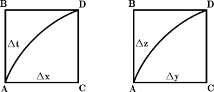
Imagine a small rectangle in spacetime with corners

$A=(0,0,0,0),\;B=(dt,0,0,0),\;C=(0,dx,0,0),\;D=(dt,dx,0,0).$

Let's calculate the electromagnetic contribution to the action of the path from $A$ to $D$ via $B$ for a unit charge ($q=1$) in natural units ( $c=1$ ):

$S_{ABD}=-V(dt/2,0,0,0)\,dt+A_{x}(dt,dx/2,0,0)\,dx$

$\quad =-V(dt/2,0,0,0)\,dt+\left[A_{x}(0,dx/2,0,0)+{\partial A_{x} \over \partial t}dt\right]dx.$

Next, the contribution to the action of the path from $A$ to $D$ via $C$:

$S_{ACD}=A_{x}(0,dx/2,0,0)\,dx-V(dt/2,dx,0,0)\,dt$

$=A_{x}(0,dx/2,0,0)\,dx-\left[V(dt/2,0,0,0)+{\partial V \over \partial x}dx\right]dt.$

Look at the difference:

$\Delta S=S_{ACD}-S_{ABD}=\left(-{\partial V \over \partial x}-{\partial A_{x} \over \partial t}\right)dt\,dx=E_{x}\,dt\,dx.$

Alternatively, you may think of $\Delta S$ as the electromagnetic contribution to the action of the loop $A\rightarrow B\rightarrow D\rightarrow C\rightarrow A.$

Let's repeat the calculation for a small rectangle with corners

$A=(0,0,0,0),\;B=(0,0,dy,0),\;C=(0,0,0,dz),\;D=(0,0,dy,dz).$

$S_{ABD}=A_{z}(0,0,0,dz/2)\,dz+A_{y}(0,0,dy/2,dz)\,dy$

$=A_{z}(0,0,0,dz/2)\,dz+\left[A_{y}(0,0,dy/2,0)+{\partial A_{y} \over \partial z}dz\right]dy,$

$S_{ACD}=A_{y}(0,0,dy/2,0)\,dy+A_{z}(0,0,dy,dz/2)\,dz$

$=A_{y}(0,0,dy/2,0)\,dy+\left[A_{z}(0,0,0,dz/2)+{\partial A_{z} \over \partial y}dy\right]dz,$

$\Delta S=S_{ACD}-S_{ABD}=\left({\partial A_{z} \over \partial y}-{\partial A_{y} \over \partial z}\right)dy\,dz=B_{x}\,dy\,dz.$

Thus the electromagnetic contribution to the action of this loop equals the flux of $\mathbf {B}$ through the loop.

Remembering (i) Stokes' theorem and (ii) the definition of $\mathbf {B}$ in terms of $\mathbf {A} ,$ we find that

$\oint _{\partial \Sigma }\mathbf {A} \cdot d\mathbf {r} =\int _{\Sigma }{\hbox{curl}}\,\mathbf {A} \cdot d\mathbf {\Sigma } =\int _{\Sigma }\mathbf {B} \cdot d\mathbf {\Sigma } .$

In (other) words, the magnetic flux through a loop $\partial \Sigma$ (or through any surface $\Sigma$ bounded by $\partial \Sigma$ ) equals the circulation of $\mathbf {A}$ around the loop (or around any surface bounded by the loop).

The effect of a circulation $\oint _{\partial \Sigma }\mathbf {A} \cdot d\mathbf {r}$ around the finite rectangle $A\rightarrow B\rightarrow D\rightarrow C\rightarrow A$ is to increase (or decrease) the action associated with the segment $A\rightarrow B\rightarrow D$ relative to the action associated with the segment $A\rightarrow C\rightarrow D.$ If the actions of the two segments are equal, then we can expect the path of least action from $A$ to $D$ to be a straight line. If one segment has a greater action than the other, then we can expect the path of least action from $A$ to $D$ to curve away from the segment with the larger action.

Compare this with the classical story, which explains the curvature of the path of a charged particle in a magnetic field by invoking a force that acts at right angles to both the magnetic field and the particle's direction of motion. The quantum-mechanical treatment of the same effect offers no such explanation. Quantum mechanics invokes no mechanism of any kind. It simply tells us that for a sufficiently massive charge traveling from $A$ to $D,$ the probability of finding that it has done so within any bundle of paths not containing the action-geodesic connecting $A$ with $D,$ is virtually 0.

Much the same goes for the classical story according to which the curvature of the path of a charged particle in a spacetime plane is due to a force that acts in the direction of the electric field. (Observe that curvature in a spacetime plane is equivalent to acceleration or deceleration. In particular, curvature in a spacetime plane containing the $x$ axis is equivalent to acceleration in a direction parallel to the $x$ axis.) In this case the corresponding circulation is that of the 4-vector potential $(cV,\mathbf {A} )$ around a spacetime loop.