Partial Differential Equations/Poisson's equation

This chapter deals with Poisson's equation

$\forall x\in \mathbb {R} ^{d}:-\Delta u(x)=f(x)$

Provided that $f\in {\mathcal {C}}^{2}(\mathbb {R} ^{d})$, we will through distribution theory prove a solution formula, and for domains with boundaries satisfying a certain property we will even show a solution formula for the boundary value problem. We will also study solutions of the homogenous Poisson's equation

$\forall x\in \mathbb {R} ^{d}:-\Delta u(x)=0$

The solutions to the homogenous Poisson's equation are called harmonic functions.

Important theorems from multi-dimensional integration

In section 2, we had seen Leibniz' integral rule, and in section 4, Fubini's theorem. In this section, we repeat the other theorems from multi-dimensional integration which we need in order to carry on with applying the theory of distributions to partial differential equations. Proofs will not be given, since understanding the proofs of these theorems is not very important for the understanding of this wikibook. The only exception will be theorem 6.3, which follows from theorem 6.2. The proof of this theorem is an exercise.

Theorem 6.2: (Divergence theorem)

Let $K\subset \mathbb {R} ^{d}$ a compact set with smooth boundary. If $\mathbf {V} :K\to \mathbb {R} ^{d}$ is a vector field, then

$\int _{K}\nabla \cdot \mathbf {V} (x)dx=\int _{\partial K}\nu (x)\cdot \mathbf {V} (x)dx$

, where $\nu :\partial K\to \mathbb {R} ^{d}$ is the outward normal vector.

Theorem 6.3: (Multi-dimensional integration by parts)

Let $K\subset \mathbb {R} ^{d}$ a compact set with smooth boundary. If $f:K\to \mathbb {R}$ is a function and $\mathbf {W} :K\to \mathbb {R} ^{d}$ is a vector field, then

$\int _{K}f(x)\nabla \cdot \mathbf {W} (x)dx=\int _{\partial K}f(x)\nu (x)\cdot \mathbf {W} (x)dx-\int _{K}\mathbf {W} (x)\cdot \nabla f(x)dx$

, where $\nu :\partial K\to \mathbb {R} ^{d}$ is the outward normal vector.

Proof: See exercise 1.

The volume and surface area of d-dimensional spheres

Definition 6.5:

The Gamma function $\Gamma :\mathbb {R} _{>0}\to \mathbb {R}$ is defined by

$\Gamma (x):=\int _{0}^{\infty }s^{x-1}e^{-s}ds$

The Gamma function satisfies the following equation:

Theorem 6.6:

$\forall x\in \mathbb {R} _{>0}:\Gamma (x+1)=x\Gamma (x)$

Proof:

$\Gamma (x+1)=\int _{0}^{\infty }s^{x}e^{-s}ds{\overset {\text{integration by parts}}{=}}\underbrace {-s^{x}e^{-s}{\big |}_{s=0}^{s=\infty }} _{=0}-\int _{0}^{\infty }-xs^{x-1}e^{-s}ds=x\Gamma (x)$

$\Box$

If the Gamma function is shifted by 1, it is an interpolation of the factorial (see exercise 2):

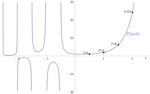
As you can see, in the above plot the Gamma function also has values on negative numbers. This is because what is plotted above is some sort of a natural continuation of the Gamma function which one can construct using complex analysis.

Definition and theorem 6.7:

The $d$-dimensional spherical coordinates, given by $\Psi :(0,\infty )\times (0,2\pi )\times (-\pi /2,\pi /2)^{d-2}\to \mathbb {R} ^{d}\setminus \{(x_{1},\ldots ,x_{d})\in \mathbb {R} ^{d}:x_{1}\geq 0\wedge x_{2}=0\}$

$\Psi (r,\Phi ,\Theta _{1},\ldots ,\Theta _{d-2})={\begin{pmatrix}r\cos(\Phi )\cos(\Theta _{1})\cdots \cos(\Theta _{d-2})\\r\sin(\Phi )\cos(\Theta _{1})\cdots \cos(\Theta _{d-2})\\r\sin(\Theta _{1})\cos(\Theta _{2})\cdots \cos(\Theta _{d-2})\\\vdots \\r\sin(\Theta _{d-3})\cos(\Theta _{d-2})\\r\sin(\Theta _{d-2})\\\end{pmatrix}}$

are a diffeomorphism. The determinant of the Jacobian matrix of $\Psi$, $\det J_{\Psi }$, is given by

$\det J_{\Psi }(r,\Phi ,\Theta _{1},\ldots ,\Theta _{d-2})=r^{d-1}\cos(\Theta _{1})\cos(\Theta _{2})^{2}\cdots \cos(\Theta _{d-2})^{d-2}$

Proof:

Theorem 6.8:

The volume of the $d$-dimensional ball with radius $R\in \mathbb {R} _{>0}$, $B_{R}(0)$ is given by

$V_{d}(R):={\frac {\pi ^{d/2}}{\Gamma (d/2+1)}}R^{d}$

Proof:

Theorem 6.9:

The area of the surface of the $d$-dimensional ball with radius $R\in \mathbb {R} _{>0}$ (i. e. the area of $\partial B_{R}(0)$) is given by

$A_{d}(R):={\frac {d\pi ^{d/2}}{\Gamma (d/2+1)}}R^{d-1}$

The surface area and the volume of the $d$-dimensional ball with radius $R\in \mathbb {R} _{>0}$ are related to each other "in a differential way" (see exercise 3).

Proof:

${\begin{aligned}A_{d}(R)&:={\frac {d\pi ^{d/2}}{\Gamma (d/2+1)}}R^{d-1}&\\&={\frac {d}{R}}V_{d}(R)&\\&={\frac {d}{R}}\int _{B_{R}(0)}1dx&{\text{ theorem 6.8}}\\&=\int _{B_{R}(0)}{\frac {1}{R}}\nabla \cdot xdx&\\&=\int _{\partial B_{R}(0)}{\frac {1}{R}}{\frac {x}{R}}\cdot xdx&{\text{ divergence theorem}}\\&=\int _{\partial B_{R}(0)}1dx&\end{aligned}}$$\Box$

Green's kernel

We recall a fact from integration theory:

Lemma 6.11: $f$ is integrable $\Leftrightarrow$ $|f|$ is integrable.

We omit the proof.

Theorem 6.12:

The function $P:\mathbb {R} ^{d}\to \mathbb {R}$, given by

$P(x):={\begin{cases}-{\frac {1}{2}}|x|&d=1\\-{\frac {1}{2\pi }}\ln(\|x\|)&d=2\\{\frac {1}{(d-2)A_{d}(1)\|x\|^{d-2}}}&d\geq 3\end{cases}}$

is a Green's kernel for Poisson's equation.

We only prove the theorem for $d\geq 2$. For $d=1$ see exercise 4.

Proof:

1.

We show that $P$ is locally integrable. Let $K\subseteq \mathbb {R} ^{d}$ be compact. We have to show that

$\int _{K}P(x)dx$

is a real number, which by lemma 6.11 is equivalent to

$\int _{K}|P(x)|dx$

is a real number. As compact in $\mathbb {R} ^{d}$ is equivalent to bounded and closed, we may choose an $R>0$ such that $K\subset B_{R}(0)$. Without loss of generality we choose $R>1$, since if it turns out that the chosen $R$ is $\leq 1$, any $R>1$ will do as well. Then we have

$\int _{K}|P(x)|dx\leq \int _{B_{R}(0)}|P(x)|dx$

For $d=2$, ${\begin{aligned}\int _{B_{R}(0)}|P(x)|dx&=\int _{B_{1}(0)}-{\frac {1}{2\pi }}\ln(\|x\|)dx+\int _{B_{R}(0)\setminus B_{1}(0)}{\frac {1}{2\pi }}\ln(\|x\|)dx&\\&=\int _{B_{1}(0)}-{\frac {1}{2\pi }}\ln(\|x\|)dx+\int _{B_{R}(0)}{\frac {1}{2\pi }}\ln(\|x\|)dx-\int _{B_{1}(0)}{\frac {1}{2\pi }}\ln(\|x\|)dx&\\&=\int _{0}^{1}-{\frac {r}{\pi }}\ln(r)dr+\int _{0}^{R}{\frac {r}{2\pi }}\ln(r)dr&{\text{int. by subst. using spherical coords.}}\\&={\frac {1}{4\pi }}+{\frac {R^{2}}{4\pi }}\left(\ln(R)-{\frac {1}{2}}R\right)<\infty \end{aligned}}$

For $d\geq 3$,

${\begin{aligned}\int _{B_{R}(0)}|P(x)|dx&=\int _{B_{R}(0)}{\frac {1}{(d-2)A_{d}(1)\|x\|^{d-2}}}\\&=\int _{0}^{R}\int _{0}^{2\pi }\underbrace {\int _{-{\frac {\pi }{2}}}^{\frac {\pi }{2}}\cdots \int _{-{\frac {\pi }{2}}}^{\frac {\pi }{2}}} _{d-2{\text{ times}}}\overbrace {|r^{d-1}\cos(\Theta _{1})\cdots \cos(\Theta _{d-2})^{d-2}|} ^{\leq r^{d-1}}{\frac {1}{(d-2)A_{d}(1)r^{d-2}}}d\Theta _{1}\cdots d\Theta _{d-2}d\Phi dr\\&\leq \int _{0}^{R}2{\frac {r^{d-1}}{(d-2)A_{d}(1)r^{d-2}}}\pi ^{d-1}dr\\&={\frac {\pi ^{d-1}}{(d-2)A_{d}(1)}}R^{2}\end{aligned}}$

, where we applied integration by substitution using spherical coordinates from the first to the second line.

2.

We calculate some derivatives of $P$ (see exercise 5):

For $d=2$, we have

$\forall x\in \mathbb {R} ^{d}\setminus \{0\}:\nabla P(x)=-{\frac {x}{2\pi \|x\|^{2}}}$

For $d\geq 3$, we have

$\forall x\in \mathbb {R} ^{d}\setminus \{0\}:\nabla P(x)={\frac {x}{A_{d}(1)\|x\|^{d}}}$

For all $d\geq 2$, we have $\forall x\in \mathbb {R} ^{d}\setminus \{0\}:\Delta P(x)=0$

3.

We show that

$\forall x\in \mathbb {R} ^{d}:-\Delta {\mathcal {T}}_{P(\cdot -x)}=\delta _{x}$

Let $x\in \mathbb {R} ^{d}$ and $\varphi \in {\mathcal {D}}(\mathbb {R} ^{d})$ be arbitrary. In this last step of the proof, we will only manipulate the term $-\Delta {\mathcal {T}}_{P(\cdot -x)}(\varphi )$. Since $\varphi \in {\mathcal {D}}(\mathbb {R} ^{d})$, $\varphi$ has compact support. Let's define

$K:={\text{supp }}\varphi \cup {\overline {B_{1}(x)}}$

Since the support of

${\begin{aligned}-\Delta {\mathcal {T}}_{P(\cdot -x)}(\varphi )&={\mathcal {T}}_{P(\cdot -x)}(-\Delta \varphi )&\\&=\int _{\mathbb {R} ^{d}}P(y-x)(-\Delta \varphi (y))dy&\\&=\int _{K}P(y-x)(-\Delta \varphi (y))dy&\\&=\lim _{\epsilon \downarrow 0}\int _{K}P(y-x)(-\Delta \varphi (y))\chi _{K\setminus B_{\epsilon }(x)}(y)dy&{\text{dominated convergence}}\\&=\lim _{\epsilon \downarrow 0}\int _{K\setminus B_{\epsilon }(x)}P(y-x)(-\Delta \varphi (y))dy&\\\end{aligned}}$

, where $\chi _{K\setminus B_{\epsilon }(0)}$ is the characteristic function of $K\setminus B_{\epsilon }(0)$.

The last integral is taken over $K\setminus B_{\epsilon }(x)$ (which is bounded and as the intersection of the closed sets $K$ and $\mathbb {R} ^{d}\setminus B_{\epsilon }(x)$ closed and thus compact as well). In this area, due to the above second part of this proof, $P(y-x)$ is continuously differentiable. Therefore, we are allowed to integrate by parts. Thus, noting that ${\frac {x-y}{\|y-x\|}}$ is the outward normal vector in $y\in \partial B_{\epsilon }(x)$ of $K\setminus B_{\epsilon }(x)$, we obtain

$\int _{K\setminus B_{\epsilon }(x)}P(y-x)\overbrace {(-\Delta \varphi (y))} {=-\nabla \cdot \nabla \varphi (y)}dy=\int _{\partial B_{\epsilon }(x)}P(y-x)\nabla \varphi (y)\cdot {\frac {x-y}{\|y-x\|}}dy-\int _{\mathbb {R} ^{d}\setminus B_{\epsilon }(x)}\nabla \varphi (y)\cdot \nabla P(y-x)dy$

Let's furthermore choose $w(x)={\tilde {G}}(x-\xi )\nabla \varphi (x)$. Then

$\nabla \cdot w(x)=\Delta \varphi (x){\tilde {G}}(x-\xi )+\langle \nabla {\tilde {G}}(x-\xi ),\nabla \varphi (x)\rangle$.

From Gauß' theorem, we obtain

$\int _{\mathbb {R} ^{d}\setminus B_{R}(\xi )}\Delta \varphi (x){\tilde {G}}(x-\xi )+\langle \nabla {\tilde {G}}(x-\xi ),\nabla \varphi (x)\rangle dx=-\int _{\partial B_{R}(\xi )}\langle {\tilde {G}}(x-\xi )\nabla \varphi (x),{\frac {x-\xi }{\|x-\xi \|}}\rangle dx$

, where the minus in the right hand side occurs because we need the inward normal vector. From this follows immediately that

$\int _{\mathbb {R} ^{d}\setminus B_{R}(\xi )}-\Delta \varphi (x){\tilde {G}}(x-\xi )=\underbrace {\int _{\partial B_{R}(\xi )}\langle {\tilde {G}}(x-\xi )\nabla \varphi (x),{\frac {x-\xi }{\|x-\xi \|}}\rangle dx} _{:=J_{1}(R)}-\underbrace {\int _{\mathbb {R} ^{d}\setminus B_{R}(\xi )}\langle \nabla {\tilde {G}}(x-\xi ),\nabla \varphi (x)\rangle dx} _{:=J_{2}(R)}$

We can now calculate the following, using the Cauchy-Schwartz inequality:

$|J_{1}(R)|\leq \int _{\partial B_{R}(\xi )}\|{\tilde {G}}(x-\xi )\nabla \varphi (x)\|\overbrace {\|{\frac {x-\xi }{\|x-\xi \|}}\|} ^{=1}dx$

$={\begin{cases}\displaystyle \int _{\partial B_{R}(\xi )}-{\frac {1}{2\pi }}\ln |x-\xi |\|\nabla \varphi (x)\|dx=\int _{\partial B_{1}(\xi )}-R{\frac {1}{2\pi }}\ln \|R(x-\xi )\|\|\nabla \varphi (Rx)\|dx&d=2\\\displaystyle \int _{\partial B_{R}(\xi )}{\frac {1}{(d-2)c}}{\frac {1}{|x-\xi |^{d-2}}}\|\nabla \varphi (x)\|dx=\int _{\partial B_{1}(\xi )}R^{d-1}{\frac {1}{(d-2)c}}{\frac {1}{|R(x-\xi )|^{d-2}}}&d\geq 3\end{cases}}$

$\leq {\begin{cases}\displaystyle \max \limits _{x\in \mathbb {R} ^{d}}\|\nabla \varphi (Rx)\|\int _{\partial B_{1}(\xi )}-R{\frac {1}{2\pi }}\ln R^{2}dx=-\max \limits _{x\in \mathbb {R} ^{d}}\|\nabla \varphi (Rx)\|{\frac {c}{2\pi }}R\ln R^{2}\to 0,R\to 0&d=2\\\displaystyle \max \limits _{x\in \mathbb {R} ^{d}}\|\nabla \varphi (Rx)\|\int _{\partial B_{1}(\xi )}{\frac {1}{(d-2)c}}Rdx=\max \limits _{x\in \mathbb {R} ^{d}}\|\nabla \varphi (Rx)\|{\frac {R}{d-2}}\to 0,R\to 0&d\geq 3\end{cases}}$

Now we define $v(x)=\varphi (x)\nabla {\tilde {G}}(x-\xi )$, which gives:

$\nabla \cdot v(x)=\varphi (x)\underbrace {\Delta {\tilde {G}}(x-\xi )} _{=0,x\neq \xi }+\langle \nabla \varphi (x),\nabla {\tilde {G}}(x-\xi )\rangle$

Applying Gauß' theorem on $v$ gives us therefore

$J_{2}(R)=\int _{\partial B_{R}(\xi )}\varphi (x)\langle \nabla {\tilde {G}}(x-\xi ),{\frac {x-\xi }{\|x-\xi \|}}\rangle dx$

$=\int _{\partial B_{R}(\xi )}\varphi (x)\langle -{\frac {x-\xi }{c\|x-\xi \|^{d}}},{\frac {x-\xi }{\|x-\xi \|}}\rangle dx=-{\frac {1}{c}}\int _{\partial B_{R}(\xi )}{\frac {1}{R^{d-1}}}\varphi (x)dx$

, noting that $d=2\Rightarrow c=2\pi$.

We furthermore note that

$\varphi (\xi )={\frac {1}{c}}\int _{\partial B_{1}(\xi )}\varphi (\xi )dx={\frac {1}{c}}\int _{\partial B_{R}(\xi )}{\frac {1}{R^{d-1}}}\varphi (\xi )dx$

Therefore, we have

$\lim _{R\to 0}|-J_{2}(R)-\varphi (\xi )|\leq {\frac {1}{c}}\lim _{R\to 0}\int _{\partial B_{R}(\xi )}{\frac {1}{R^{d-1}}}|\varphi (\xi )-\varphi (x)|dx\leq \lim _{R\to 0}{\frac {1}{c}}\max _{x\in B_{R}(\xi )}|\varphi (x)-\varphi (\xi )|\int _{\partial B_{1}(\xi )}1dx$

$=\lim _{R\to 0}\max _{x\in B_{R}(\xi )}|\varphi (x)-\varphi (\xi )|=0$

due to the continuity of $\varphi$.

Thus we can conclude that

$\forall \Omega {\text{ domain of }}\mathbb {R} ^{d}:\forall \varphi \in {\mathcal {D}}(\Omega ):-\Delta T_{{\tilde {G}}(\cdot -\xi )}(\varphi )=\lim _{R\to 0}J_{0}(R)=\lim _{R\to 0}J_{1}(R)-J_{2}(R)=0+\varphi (\xi )=\delta _{\xi }(\varphi )$.

Therefore, ${\tilde {G}}$ is a Green's kernel for the Poisson's equation for $d\geq 2$.

QED.

Integration over spheres

Theorem 6.12:

Let $f:\mathbb {R} ^{d}\to \mathbb {R}$ be a function. $\int _{\partial B_{R}(0)}f(x)dx=R^{d-1}\int _{0}^{2\pi }\underbrace {\int _{-{\frac {\pi }{2}}}^{\frac {\pi }{2}}\cdots \int _{-{\frac {\pi }{2}}}^{\frac {\pi }{2}}} _{d-2{\text{ times}}}f\left(\Psi (r,\Phi ,\Theta _{1},\ldots ,\Theta _{d-2})\right)\cos(\Theta _{1})\cos(\Theta _{2})^{2}\cdots \cos(\Theta _{d-2})^{d-2}d\Theta _{1}d\Theta _{2}\cdots d\Theta _{d-2}d\Phi$

Proof: We choose as an orientation the border orientation of the sphere. We know that for $\partial B_{r}(0)$, an outward normal vector field is given by $\nu (x)={\frac {x}{r}}$. As a parametrisation of $B_{r}(0)$, we only choose the identity function, obtaining that the basis for the tangent space there is the standard basis, which in turn means that the volume form of $B_{r}(0)$ is

$\omega _{B_{r}(0)}(x)=e_{1}^{*}\wedge \cdots \wedge e_{d}^{*}$

Now, we use the normal vector field to obtain the volume form of $\partial B_{r}(0)$:

$\omega _{\partial B_{r}(0)}(x)(v_{1},\ldots ,v_{d-1})=\omega _{B_{r}(0)}(x)(\nu (x),v_{1},\ldots ,v_{d-1})$

We insert the formula for $\omega _{B_{r}(0)}(x)$ and then use Laplace's determinant formula:

$=e_{1}^{*}\wedge \cdots \wedge e_{d}^{*}(\nu (x),v_{1},\ldots ,v_{d-1})={\frac {1}{r}}\sum _{i=1}^{d}(-1)^{i+1}x_{i}e_{1}^{*}\cdots \wedge e_{i-1}^{*}\wedge e_{i+1}^{*}\wedge \cdots \wedge e_{d}^{*}(v_{1},\ldots ,v_{d-1})$

As a parametrisation of $\partial B_{r}(x)$ we choose spherical coordinates with constant radius $r$.

We calculate the Jacobian matrix for the spherical coordinates:

$J=\left({\begin{smallmatrix}\cos(\varphi )\cos(\vartheta _{1})\cdots \cos(\vartheta _{d-2})&r-\sin(\varphi )\cos(\vartheta _{1})\cdots \cos(\vartheta _{d-2})&-r\cos(\varphi )\sin(\vartheta _{1})\cdots \cos(\vartheta _{d-2})&\cdots &\cdots &-r\cos(\varphi )\cos(\vartheta _{1})\cdots \sin(\vartheta _{d-2})\\\sin(\varphi )\cos(\vartheta _{1})\cdots \cos(\vartheta _{d-2})&r\cos(\varphi )\cos(\vartheta _{1})\cdots \cos(\vartheta _{d-2})&-r\sin(\varphi )\sin(\vartheta _{1})\cdots \cos(\vartheta _{d-2})&\cdots &\cdots &-r\sin(\varphi )\cos(\vartheta _{1})\cdots \sin(\vartheta _{d-2})\\\vdots &0&\ddots &\ddots &\ddots &\vdots \\\vdots &\vdots &\ddots &\ddots &\ddots &\\\sin(\vartheta _{d-3})\cos(\vartheta _{d-2})&0&\cdots &0&r\cos(\vartheta _{d-3})\cos(\vartheta _{d-2})&r\sin(\vartheta _{d-3})\cos(\vartheta _{d-2})\\\sin(\vartheta _{d-2})&0&\cdots &\cdots &0&r\cos(\vartheta _{d-2})\end{smallmatrix}}\right)$

We observe that in the first column, we have only the spherical coordinates divided by $r$. If we fix $r$, the first column disappears. Let's call the resulting matrix $J'$ and our parametrisation, namely spherical coordinates with constant $r$, $\Psi$. Then we have:

$\Psi ^{*}\omega _{\partial B_{r}(0)}(x)(v_{1},\ldots ,v_{d-1})=\omega _{\partial B_{r}(0)}(\Psi (x))(J'v_{1},\ldots ,J'v_{d-1})$

$={\frac {1}{r}}\sum _{i=1}^{d}(-1)^{i+1}\Psi (x)_{i}e_{1}^{*}\cdots \wedge e_{i-1}^{*}\wedge e_{i+1}^{*}\wedge \cdots \wedge e_{d}^{*}(J'v_{1},\ldots ,J'v_{d-1})$

$={\frac {1}{r}}\sum _{i=1}^{d}(-1)^{i+1}\Psi (x)_{i}\det(e_{j}^{*}(J'v_{k}))_{j\neq i}=\det J\cdot \det(v_{1},\ldots ,v_{d-1})$

Recalling that

$\det J=r^{d-1}\cos(\phi _{1})^{n-2}\cos(\phi _{2})^{d-3}\cdots \cos(\phi _{d-2})$

, the claim follows using the definition of the surface integral.

Theorem 6.13:

Let $f:\mathbb {R} ^{d}\to \mathbb {R}$ be a function. Then

$\int _{\mathbb {R} ^{d}}f(x)dx=\int _{0}^{\infty }r^{d-1}\int _{\partial B_{1}(0)}f(rx)dxdr$

Proof:

We have $r\Psi (1,\Phi ,\Theta _{1},\ldots ,\Theta _{d-2})=\Psi (r,\Phi ,\Theta _{1},\ldots ,\Theta _{d-2})$, where $\Psi$ are the spherical coordinates. Therefore, by integration by substitution, Fubini's theorem and the above formula for integration over the unit sphere,

${\begin{aligned}\int _{\mathbb {R} ^{d}}f(x)dx&=\int _{(0,\infty )\times (0,2\pi )\times (-\pi /2,\pi /2)^{d-2}}f(\Psi (x))|\det J_{\Psi }(x)|dx\\&=\int _{0}^{\infty }\int _{0}^{2\pi }\underbrace {\int _{-{\frac {\pi }{2}}}^{\frac {\pi }{2}}\cdots \int _{-{\frac {\pi }{2}}}^{\frac {\pi }{2}}} _{d-2{\text{ times}}}f(\Psi (r,\Phi ,\Theta _{1},\ldots ,\Theta _{d-2}))r^{d-1}\cos(\Theta _{1})\cdots \cos(\Theta _{d-2})^{d-2}d\Theta _{1}\cdots d\Theta _{d-2}d\Phi dr\\&=\int _{0}^{\infty }r^{d-1}\int _{0}^{2\pi }\underbrace {\int _{-{\frac {\pi }{2}}}^{\frac {\pi }{2}}\cdots \int _{-{\frac {\pi }{2}}}^{\frac {\pi }{2}}} _{d-2{\text{ times}}}f(r\Psi (1,\Phi ,\Theta _{1},\ldots ,\Theta _{d-2}))\cos(\Theta _{1})\cdots \cos(\Theta _{d-2})^{d-2}d\Theta _{1}\cdots d\Theta _{d-2}d\Phi dr\\&=\int _{0}^{\infty }r^{d-1}\int _{\partial B_{1}(0)}f(rx)dr\end{aligned}}$$\Box$

Harmonic functions

Definition 6.14: Let $O\subseteq \mathbb {R} ^{d}$ be open and let $u:O\to \mathbb {R}$ be a function. If $u\in {\mathcal {C}}^{2}(O)$ and

$\forall x\in O:\Delta u(x)=0$

$u$ is called a harmonic function.

Theorem 6.15:

Let $O\subseteq \mathbb {R} ^{d}$ be open and let $u\in {\mathcal {C}}^{2}(O)$. The following conditions are equivalent:

• $u$ is harmonic
• $\forall x\in O:\forall R{\text{ such that }}{\overline {B_{R}(0)}}\subset O:u(x)={\frac {1}{A_{d}(R)}}\int _{\partial B_{R}(x)}u(y)dy$
• $\forall x\in O:\forall R{\text{ such that }}{\overline {B_{R}(0)}}\subset O:u(x)={\frac {1}{V_{d}(R)}}\int _{B_{R}(x)}u(y)dy$

Proof: Let's define the following function:

$\phi (r)={\frac {1}{r^{d-1}}}\int _{\partial B_{r}(x)}u(y)dy$

From first coordinate transformation with the diffeomorphism $y\mapsto x+y$ and then applying our formula for integration on the unit sphere twice, we obtain:

$\phi (r)={\frac {1}{r^{d-1}}}\int _{\partial B_{r}(0)}u(y+x)dy=\int _{\partial B_{1}(0)}u(x+ry)dy$

From first differentiation under the integral sign and then Gauss' theorem, we know that

$\phi '(r)=\int _{\partial B_{1}(0)}\langle \nabla u(x+ry),y\rangle dy=\int _{B_{1}(0)}\Delta u(x+ry)dy=0$

Case 1: If $u$ is harmonic, then we have

$\int _{B_{1}(0)}\Delta u(x+ry)dy=0$

, which is why $\phi$ is constant. Now we can use the dominated convergence theorem for the following calculation:

$\lim _{r\to 0}\phi (r)=\int _{\partial B_{1}(0)}\lim _{r\to 0}u(x+ry)dy=c(1)u(x)$

Therefore $\phi (r)=c(1)u(x)$ for all $r$.

With the relationship

$r^{d-1}c(1)=c(r)$

, which is true because of our formula for $c(x),x\in \mathbb {R} _{>0}$, we obtain that

$u(x)={\frac {\phi (r)}{c(1)}}={\frac {1}{c(1)}}{\frac {1}{r^{d-1}}}\int _{\partial B_{r}(x)}u(y)dy={\frac {1}{c(r)}}\int _{\partial B_{r}(x)}u(y)dy$

, which proves the first formula.

Furthermore, we can prove the second formula by first transformation of variables, then integrating by onion skins, then using the first formula of this theorem and then integration by onion skins again:

$\int _{B_{r}(x)}u(y)dy=\int _{B_{r}(0)}u(y+x)dy=\int _{0}^{r}s^{d-1}\int _{\partial B_{1}(0)}u(y+sx)dxds=\int _{0}^{r}s^{d-1}u(x)\int _{\partial B_{1}(0)}1dxds=u(x)d(r)$

This shows that if $u$ is harmonic, then the two formulas for calculating $u$, hold.

Case 2: Suppose that $u$ is not harmonic. Then there exists an $x\in \Omega$ such that $-\Delta u(x)\neq 0$. Without loss of generality, we assume that $-\Delta u(x)>0$; the proof for $-\Delta u(x)<0$ will be completely analogous exept that the direction of the inequalities will interchange. Then, since as above, due to the dominated convergence theorem, we have

$\lim _{r\to 0}\phi '(r)=\int _{B_{1}(0)}\lim _{r\to 0}\Delta u(x+ry)dy>0$

Since $\phi '$ is continuous (by the dominated convergence theorem), this is why $\phi$ grows at $0$, which is a contradiction to the first formula.

The contradiction to the second formula can be obtained by observing that $\phi '$ is continuous and therefore there exists a $\sigma \in \mathbb {R} _{>0}$

$\forall r\in [0,\sigma ):\phi '(r)>0$

This means that since

$\lim _{r\to 0}\phi (r)=\int _{\partial B_{1}(0)}\lim _{r\to 0}u(x+ry)dy=c(1)u(x)$

and therefore

$\phi (0)=c(1)u(x)$

, that

$\forall r\in (0,\sigma ):\phi (r)>c(1)u(x)$

and therefore, by the same calculation as above,

$\int _{B_{r}(x)}u(y)dy=\int _{B_{r}(0)}u(y+x)dy=\int _{0}^{r}s^{d-1}\int _{\partial B_{1}(0)}u(y+sx)dxds>\int _{0}^{r}s^{d-1}u(x)\int _{\partial B_{1}(0)}1dxds=u(x)d(r)$

This shows (by proof with contradiction) that if one of the two formulas hold, then $u\in C^{2}(\Omega )$ is harmonic.

Definition 6.16:

A domain is an open and connected subset of $\mathbb {R} ^{d}$.

For the proof of the next theorem, we need two theorems from other subjects, the first from integration theory and the second from topology.

Theorem 6.17:

Let $B\subseteq \mathbb {R} ^{d}$ and let $f:B\to \mathbb {R}$ be a function. If

$\int _{B}|f(x)|dx=0$

then $f(x)=0$ for almost every $x\in B$.

Theorem 6.18:

In a connected topological space, the only simultaneously open and closed sets are the whole space and the empty set.

We will omit the proofs.

Theorem 6.19:

Let $\Omega \subseteq \mathbb {R} ^{d}$ be a domain and let $u:\Omega \to \mathbb {R}$ be harmonic. If there exists an $x\in \Omega$ such that

$u(x)=\sup _{y\in \Omega }u(y)$

, then $u$ is constant.

Proof:

We choose

$B:=\left\{x\in \Omega :u(x)=\sup _{y\in \Omega }u(y)\right\}$

Since $\Omega$ is open by assumption and $B\subseteq \Omega$, for every $x\in B$ exists an $R\in \mathbb {R} _{>0}$ such that

${\overline {B_{R}(x)}}\subseteq \Omega$

By theorem 6.15, we obtain in this case:

$\sup _{y\in \Omega }u(y)=u(x)={\frac {1}{V_{d}(R)}}\int _{B_{R}(x)}u(z)dz$

Further,

$\sup _{y\in \Omega }u(y)=\sup _{y\in \Omega }u(y){\frac {V_{d}(R)}{V_{d}(R)}}={\frac {1}{V_{d}(R)}}\int _{B_{r}(x)}\sup _{y\in \Omega }u(y)dz$

, which is why

${\begin{aligned}{\frac {1}{V_{d}(R)}}\int _{B_{R}(x)}u(z)dz=\int _{B_{R}(x)}\sup _{y\in \Omega }u(y)dz\\\Leftrightarrow {\frac {1}{V_{d}(R)}}\int _{B_{R}(x)}(u(z)-\sup _{y\in \Omega }u(y))dz=0\end{aligned}}$

Since

$\forall z\in \Omega :\sup _{y\in \Omega }u(y)\geq u(z)$

, we have even

$0={\frac {1}{V_{d}(R)}}\int _{B_{R}(x)}(u(z)-\sup _{y\in \Omega }u(y))dz=-{\frac {1}{V_{d}(R)}}\int _{B_{R}(x)}|u(z)-\sup _{y\in \Omega }u(y)|dz$

By theorem 6.17 we conclude that

$u(z)=\sup _{y\in \Omega }u(y)$

almost everywhere in $B_{R}(x)$, and since

$z\mapsto u(z)-\sup _{y\in \Omega }u(y)$

is continuous, even

$u(z)=\sup _{y\in \Omega }u(y)$

really everywhere in $B_{R}(x)$ (see exercise 6). Therefore $B_{R}(0)\subseteq B$, and since $x\in B$ was arbitrary, $B$ is open.

Also,

$B=u^{-1}\left(\left\{\sup _{y\in \Omega }u(y)\right\}\right)$

and $u$ is continuous. Thus, as a one-point set is closed, lemma 3.13 says $B$ is closed in $\Omega$. Thus $B$ is simultaneously open and closed. By theorem 6.18, we obtain that either $B=\emptyset$ or $B=\Omega$. And since by assumtion $B$ is not empty, we have $B=\Omega$.$\Box$

Theorem 6.18:

Let $\Omega \subseteq \mathbb {R} ^{d}$ be a domain and let $u:\Omega \to \mathbb {R}$ be harmonic. If there exists an $x\in \Omega$ such that

$u(x)=\inf _{y\in \Omega }u(y)$

, then $u$ is constant.

Proof: See exercise 7.

Corollary 6.20:

Let $\Omega \subseteq \mathbb {R} ^{d}$ be a bounded domain and let $u:{\overline {\Omega }}\to \mathbb {R}$ be harmonic on $\Omega$ and continuous on ${\overline {\Omega }}$. Then

$\forall x\in {\overline {\Omega }}:\inf _{y\in \partial \Omega }u(y)\leq u(x)\leq \sup _{y\in \partial \Omega }u(y)$

Proof:

Theorem 6.20:

Let $O\subseteq \mathbb {R} ^{d}$ be open and $u:O\to \mathbb {R}$ be a harmonic function, let $x_{0}\in O$ and let $R>0$ such that ${\overline {B_{R}(x_{0})}}\subset O$. Then

$\forall x\in B_{R}(x_{0}):u(x)={\frac {R^{2}+\|x-x_{0}\|^{2}}{RA_{d}(1)}}\int _{\partial B_{R}(x_{0})}{\frac {u(y)}{\|x-y\|^{d}}}dy$

Proof:

What we will do next is showing that every harmonic function $u\in {\mathcal {C}}^{2}(O)$ is in fact automatically contained in ${\mathcal {C}}^{\infty }(O)$.

Theorem 6.25: Let $O\subseteq \mathbb {R} ^{d}$ be open, and let $u:O\to \mathbb {R}$ be harmonic. Then $u\in {\mathcal {C}}^{\infty }(O)$. Furthermore, for all $n\in \mathbb {N}$, there is a constant $C_{d,n}$ depending only on the dimension $d$ and $n$ such that for all $x_{0}\in O$ and $R>0$ such that $B_{R}(x_{0})\subseteq O$

$\forall \alpha \in \mathbb {N} ^{d}{\text{ with }}|\alpha |=n:\partial _{\alpha }u(x)\leq {\frac {C_{d,n}}{R^{d+n}}}\int _{B_{R}(x_{0})}|u(y)|dy$

Proof:

Definition 6.26:

Let $(u_{l})_{l\in \mathbb {N} }$ be a sequence of harmonic functions, and let $u:O\to \mathbb {R}$ be a function. $(u_{l})_{l\in \mathbb {N} }$ converges locally uniformly to $u$ iff

Theorem 6.27:

Let $O\subseteq \mathbb {R} ^{d}$ be open and let $u_{l}:O\to \mathbb {R} ,l\in \mathbb {N}$ be harmonic functions such that the sequence $(u_{l})_{l\in \mathbb {N} }$ converges locally uniformly to a function $u:O\to \mathbb {R}$. Then also $u$ is harmonic.

Proof:

Definition 6.28:

Theorem 6.29: (Arzelà-Ascoli) Let $F$ be a set of continuous functions, which are defined on a compact set $K$. Then the following two statements are equivalent:

1. ${\overline {F}}$ (the closure of $F$) is compact
2. $F$ is bounded and equicontinuous

Proof:

Definition 6.30:

Theorem 6.31:

Let $(u_{l})_{l\in \mathbb {N} }$ be a locally uniformly bounded sequence of harmonic functions. Then it has a locally uniformly convergent subsequence.

Proof:

Boundary value problem

The dirichlet problem for the Poisson equation is to find a solution for

${\begin{cases}-\Delta u(x)=f(x)&x\in \Omega \\u(x)=g(x)&x\in \partial \Omega \end{cases}}$

Uniqueness of solutions

If $\Omega$ is bounded, then we can know that if the problem

${\begin{cases}-\Delta u(x)=f(x)&x\in \Omega \\u(x)=g(x)&x\in \partial \Omega \end{cases}}$

has a solution $u_{1}$, then this solution is unique on $\Omega$.

Proof: Let $u_{2}$ be another solution. If we define $u=u_{1}-u_{2}$, then $u$ obviously solves the problem

${\begin{cases}-\Delta u(x)=0&,x\in \Omega \\u(x)=0&x\in \partial \Omega \end{cases}}$

, since $-\Delta (u_{1}(x)-u_{2}(x))=-\Delta u_{1}(x)-(-\Delta u_{2}(x))=f(x)-f(x)=0$ for $x\in \Omega$ and $u_{1}(x)-u_{2}(x)=g(x)-g(x)=0$ for $x\in \partial \Omega$.

Due to the above corollary from the minimum and maximum principle, we obtain that $u$ is constantly zero not only on the boundary, but on the whole domain $\Omega$. Therefore $u_{1}(x)-u_{2}(x)=0\Leftrightarrow u_{1}(x)=u_{2}(x)$ on $\Omega$. This is what we wanted to prove.

Green's functions of the first kind

Let $\Omega \subseteq \mathbb {R} ^{d}$ be a domain. Let ${\tilde {G}}$ be the Green's kernel of Poisson's equation, which we have calculated above, i.e.

${\tilde {G}}(x):={\begin{cases}-{\frac {1}{2}}|x|&d=1\\-{\frac {1}{2\pi }}\ln \|x\|&d=2\\{\frac {1}{(d-2)c}}{\frac {1}{\|x\|^{d-2}}}&d\geq 3\end{cases}}$

, where $c:=\int _{\partial B_{1}(0)}1dz$ denotes the surface area of $B_{1}(0)\subset \mathbb {R} ^{d}$.

Suppose there is a function $h:\Omega \times \Omega \to \mathbb {R}$ which satisfies

${\begin{cases}-\Delta h(x,\xi )=0&x\in \Omega \\h(x,\xi )={\tilde {G}}(x-\xi )&x\in \partial \Omega \end{cases}}$

Then the Green's function of the first kind for $-\Delta$ for $\Omega$ is defined as follows:

${\tilde {G}}_{\Omega }(x,\xi ):={\tilde {G}}(x-\xi )-h(x,\xi )$

${\tilde {G}}(x-\xi )-h(x,\xi )$ is automatically a Green's function for $-\Delta$. This is verified exactly the same way as veryfying that ${\tilde {G}}$ is a Green's kernel. The only additional thing we need to know is that $h$ does not play any role in the limit processes because it is bounded.

A property of this function is that it satisfies

${\begin{cases}-\Delta {\tilde {G}}_{\Omega }(x,\xi )=0&x\in \Omega \setminus \{\xi \}\\{\tilde {G}}_{\Omega }(x,\xi )=0&x\in \partial \Omega \end{cases}}$

The second of these equations is clear from the definition, and the first follows recalling that we calculated above (where we calculated the Green's kernel), that $\Delta {\tilde {G}}(x)=0$ for $x\neq 0$.

Representation formula

Let $\Omega \subseteq \mathbb {R} ^{d}$ be a domain, and let $u\in C^{2}(\Omega )$ be a solution to the Dirichlet problem

${\begin{cases}-\Delta u(x)=f(x)&x\in \Omega \\u(x)=g(x)&x\in \partial \Omega \end{cases}}$

. Then the following representation formula for $u$ holds:

$u(\xi )=\int _{\Omega }-\Delta u(y){\tilde {G}}_{\Omega }(y,\xi )dy-\int _{\partial \Omega }u(y)\nu (y)\nabla _{y}{\tilde {G}}_{\Omega }(y,\xi )dy$

, where ${\tilde {G}}_{\Omega }$ is a Green's function of the first kind for $\Omega$.

Proof: Let's define

$J(\epsilon ):=\int _{\Omega \setminus B_{\epsilon }(\xi )}-\Delta u(y){\tilde {G}}_{\Omega }(y,\xi )dy$

. By the theorem of dominated convergence, we have that

$\lim _{\epsilon \to 0}J(\epsilon )=\int _{\Omega }-\Delta u(y){\tilde {G}}_{\Omega }(y,\xi )dy$

Using multi-dimensional integration by parts, it can be obtained that:

$J(\epsilon )=-\int _{\partial \Omega }\underbrace {{\tilde {G}}_{\Omega }(y,\xi )} _{=0}\langle \nabla u(y),\nu (y)\rangle dy+\int _{\partial B_{\epsilon }(\xi )}{\tilde {G}}_{\Omega }(y,\xi )\langle \nabla u(y),{\frac {y-\xi }{\|y-\xi \|}}\rangle dy+\int _{\Omega \setminus B_{\epsilon }(\xi )}\langle \nabla u(y),\nabla _{x}{\tilde {G}}_{\Omega }(y,\xi )\rangle dy$

$=\underbrace {\int _{\partial B_{\epsilon }(\xi )}{\tilde {G}}_{\Omega }(y,\xi )\langle \nabla u(y),{\frac {y-\xi }{\|y-\xi \|}}\rangle dy} _{:=J_{1}(\epsilon )}-\int _{\Omega \setminus B_{\epsilon }(\xi )}\Delta {\tilde {G}}_{\Omega }(y,\xi )u(y)dy$

$-\underbrace {\int _{\partial B_{\epsilon }(\xi )}u(y)\langle \nabla {\tilde {G}}_{\Omega }(y,\xi ),{\frac {y-\xi }{\|y-\xi \|}}\rangle dy} _{:=J_{2}(\epsilon )}-\int _{\partial \Omega }u(y)\langle \nabla {\tilde {G}}_{\Omega }(y,\xi ),\nu (y)\rangle dy$

When we proved the formula for the Green's kernel of Poisson's equation, we had already shown that

$\lim _{\epsilon \to 0}-J_{2}(\epsilon )=u(\xi )$ and

$\lim _{\epsilon \to 0}J_{1}(\epsilon )=0$

The only additional thing which is needed to verify this is that $h\in C^{\infty }(\Omega )$, which is why it stays bounded, while ${\tilde {G}}$ goes to infinity as $\epsilon \to 0$, which is why $h$ doesn't play a role in the limit process.

This proves the formula.

Harmonic functions on the ball: A special case of the Dirichlet problem

Green's function of the first kind for the ball

Let's choose

$h(x,\xi )={\tilde {G}}\left({\frac {\|\xi \|}{r}}\left(x-{\frac {r^{2}}{\|\xi \|^{2}}}\xi \right)\right)$

Then

${\tilde {G}}_{B_{r}(x_{0})}(x,\xi ):={\tilde {G}}(x-\xi )-h(x-x_{0},\xi -x_{0})$

is a Green's function of the first kind for $B_{r}(x_{0})$.

Proof: Since $\xi -x_{0}\in B_{r}(0)\Rightarrow {\frac {r^{2}}{\|\xi -x_{0}\|^{2}}}(\xi -x_{0})\notin B_{r}(0)$ and therefore

$\forall x,\xi \in B_{r}(0):-\Delta _{x}h(x-x_{0},\xi -x_{0})=0$

Furthermore, we obtain:

$\int _{B_{r}(x_{0})}-\Delta \varphi (x){\tilde {G}}_{\Omega }(x,\xi )dx=\int _{B_{r}(x_{0})}-\Delta \varphi (x){\tilde {G}}(x-\xi )dx+\int _{B_{r}(x_{0})}\varphi (x)-\Delta h(x,\xi )dx=\varphi (\xi )+0$

, which is why ${\tilde {G}}_{\Omega }(x,\xi )$ is a Green's function.

The property for the boundary comes from the following calculation:

$\forall x\in \partial B_{r}(0):\|x-\xi \|^{2}=\langle x-\xi ,x-\xi \rangle =r^{2}+\|\xi \|^{2}-2\langle x,\xi \rangle ={\frac {\|\xi \|^{2}}{r^{2}}}(\langle x-{\frac {r^{2}}{\|\xi \|^{2}}}\xi ,x-{\frac {r^{2}}{\|\xi \|^{2}}}\xi \rangle )={\frac {\|\xi \|^{2}}{r^{2}}}\|x-{\frac {r^{2}}{\|\xi \|^{2}}}\xi \|^{2}$

, which is why $x\in \partial B_{r}(0)\Rightarrow h(x,\xi )={\tilde {G}}(x,\xi )$, since ${\tilde {G}}$ is radially symmetric.

Solution formula

Let's consider the following problem:

${\begin{cases}-\Delta u(x)=0&x\in B_{r}(0)\\u(x)=\varphi (x)&x\in \partial B_{r}(0)\end{cases}}$

Here $\varphi$ shall be continuous on $\partial B_{r}(0)$. Then the following holds: The unique solution $u\in C({\overline {B_{r}(0)}})\cap C^{2}(B_{r}(0))$ for this problem is given by:

$u(\xi )={\begin{cases}\int _{\partial B_{r}(0)}\langle -\nu (y),\nabla _{y}{\tilde {G}}_{B_{r}(0)}(y,\xi )\rangle \varphi (y)dy&\xi \in B_{r}(0)\\\varphi (\xi )&\xi \in \partial B_{r}(0)\end{cases}}$

Proof: Uniqueness we have already proven; we have shown that for all Dirichlet problems for $-\Delta$ on bounded domains (and the unit ball is of course bounded), the solutions are unique.

Therefore, it only remains to show that the above function is a solution to the problem. To do so, we note first that

$-\Delta \int _{\partial B_{r}(0)}\langle -\nu (y),{\tilde {\nabla }}_{y}G_{B_{r}(0)}(y,\xi )\rangle \varphi (y)dy=-\Delta \int _{\partial B_{r}(0)}\langle -\nu (y),\nabla _{y}({\tilde {G}}(y-\xi )-h(y,\xi ))\rangle \varphi (y)dy$

Let $0<s<r$ be arbitrary. Since ${\tilde {G}}_{B_{r}(0)}$ is continuous in $B_{s}(0)$, we have that on $B_{s}(0)$ it is bounded. Therefore, by the fundamental estimate, we know that the integral is bounded, since the sphere, the set over which is integrated, is a bounded set, and therefore the whole integral must be always below a certain constant. But this means, that we are allowed to differentiate under the integral sign on $B_{s}(0)$, and since $r>s>0$ was arbitrary, we can directly conclude that on $B_{r}(0)$,

$-\Delta u(\xi )=\int _{\partial B_{r}(0)}\overbrace {-\Delta (\langle -\nu (y),{\tilde {\nabla }}_{y}{\tilde {G}}(x-\xi )-h(x,\xi )\rangle \varphi (y))} ^{=0}dy=0$

Furthermore, we have to show that $\forall x\in \partial B_{r}(0):\lim _{y\to x}u(y)=\varphi (x)$, i. e. that $u$ is continuous on the boundary.

To do this, we notice first that

$\int _{\partial B_{r}(0)}\langle -\nu (y),\nabla _{y}{\tilde {G}}_{B_{r}(0)}(y,\xi )\rangle dy=1$

This follows due to the fact that if $u\equiv 1$, then $u$ solves the problem

${\begin{cases}-\Delta u(x)=0&x\in B_{r}(0)\\u(x)=1&x\in \partial B_{r}(0)\end{cases}}$

and the application of the representation formula.

Furthermore, if $\|x-x^{*}\|<{\frac {1}{2}}\delta$ and $\|y-x^{*}\|\geq \delta$, we have due to the second triangle inequality:

$\|x-y\|\geq |\|y-x^{*}\|-\|x^{*}-x\||\geq {\frac {1}{2}}\delta$

In addition, another application of the second triangle inequality gives:

$(r^{2}-\|x\|^{2})=(r+\|x\|)(r-\|x\|)=(r+\|x\|)(\|x^{*}\|-\|x\|)\leq 2r\|x^{*}-x\|$

Let then $\epsilon >0$ be arbitrary, and let $x^{*}\in \partial B_{r}(0)$. Then, due to the continuity of $\varphi$, we are allowed to choose $\delta >0$ such that

$\|x-x^{*}\|<\delta \Rightarrow |\varphi (x)-\varphi (x^{*})|<{\frac {\epsilon }{2}}$.

In the end, with the help of all the previous estimations we have made, we may unleash the last chain of inequalities which shows that the representation formula is true:

$|u(x)-u(x^{*})|=|u(x)-1\cdot \varphi (x^{*})|=\left|\int _{\partial B_{r}(0)}\langle -\nu (y),\nabla _{y}{\tilde {G}}_{B_{r}(0)}(y,x)\rangle (\varphi (x)-\varphi (x^{*}))dy\right|$

$\leq {\frac {\epsilon }{2}}\int _{\partial B_{r}(0)\cap B_{\delta }(x^{*})}|\langle -\nu (y),\nabla _{y}{\tilde {G}}_{B_{r}(0)}(y,x)\rangle |dy+2\|\varphi \|_{\infty }\int _{\partial B_{r}(0)\setminus B_{\delta }(x^{*})}|\langle -\nu (y),\nabla _{y}{\tilde {G}}_{B_{r}(0)}(y,x)\rangle |dy$

$\leq {\frac {\epsilon }{2}}+2\|\varphi \|_{\infty }\int _{\partial B_{r}(0)\setminus B_{\delta }(x^{*})}{\frac {r^{2}-\|x\|^{2}}{rc(1)\left({\frac {\delta }{2}}\right)^{d}}}dy\leq {\frac {\epsilon }{2}}+2\|\varphi \|_{\infty }r^{d-2}{\frac {r^{2}-\|x\|^{2}}{\left({\frac {\delta }{2}}\right)^{d}}}$

Since $x\to x^{*}$ implies $r^{2}-\|x\|^{2}\to 0$, we might choose $x$ close enough to $x^{*}$ such that

$2\|\varphi \|_{\infty }r^{d-2}{\frac {r^{2}-\|x\|^{2}}{\left({\frac {\delta }{2}}\right)^{d}}}<{\frac {\epsilon }{2}}$. Since $\epsilon >0$ was arbitrary, this finishes the proof.

Barriers

Let $\Omega \subset \mathbb {R} ^{d}$ be a domain. A function $b:\mathbb {R} ^{d}\to \mathbb {R}$ is called a barrier with respect to $y\in \partial \Omega$ if and only if the following properties are satisfied:

1. $b$ is continuous
2. $b$ is superharmonic on $\Omega$
3. $b(y)=0$
4. $\forall x\in \mathbb {R} ^{d}\setminus \Omega :b(x)>0$

Exterior sphere condition

Let $\Omega \subseteq \mathbb {R} ^{d}$ be a domain. We say that it satisfies the exterior sphere condition, if and only if for all $x\in \partial \Omega$ there is a ball $B_{r}(z)\subseteq \mathbb {R} ^{d}\setminus \Omega$ such that $x\in \partial B_{r}(z)$ for some $z\in \mathbb {R} ^{d}\setminus \Omega$ and $r\in \mathbb {R} _{\geq 0}$.

Subharmonic and superharmonic functions

Let $\Omega \subseteq \mathbb {R} ^{d}$ be a domain and $v\in C(\Omega )$.

We call $v$ subharmonic if and only if:

$v(x)\leq {\frac {1}{d(r)}}\int _{B_{r}(x)}v(y)dy$

We call $v$ superharmonic if and only if:

$v(x)\geq {\frac {1}{d(r)}}\int _{B_{r}(x)}v(y)dy$

From this definition we can see that a function is harmonic if and only if it is subharmonic and superharmonic.

Minimum principle for superharmonic functions

A superharmonic function $u$ on $\Omega$ attains it's minimum on $\Omega$'s border $\partial \Omega$.

Proof: Almost the same as the proof of the minimum and maximum principle for harmonic functions. As an exercise, you might try to prove this minimum principle yourself.

Harmonic lowering

Let $u\in {\mathcal {S}}_{\varphi }(\Omega )$, and let $B_{r}(x_{0})\subset \Omega$. If we define

${\tilde {u}}(x)={\begin{cases}u(x)&x\notin B_{r}(x_{0})\\\int _{\partial B_{r}(0)}\langle -\nu (y),\nabla _{y}{\tilde {G}}_{B_{r}(0)}(y,x)\rangle \varphi (y)dy&x\in B_{r}(x_{0})\end{cases}}$

, then ${\tilde {u}}\in {\mathcal {S}}_{\varphi }(\Omega )$.

Proof: For this proof, the very important thing to notice is that the formula for ${\tilde {u}}$ inside $B_{r}(x_{0})$ is nothing but the solution formula for the Dirichlet problem on the ball. Therefore, we immediately obtain that ${\tilde {u}}$ is superharmonic, and furthermore, the values on $\partial \Omega$ don't change, which is why ${\tilde {u}}\in {\mathcal {S}}_{\varphi }(\Omega )$. This was to show.

Definition 3.1

Let $\varphi \in C(\partial \Omega )$. Then we define the following set:

${\mathcal {S}}_{\varphi }(\Omega ):=\{u\in C({\overline {\Omega }}):u{\text{ superharmonic and }}x\in \partial \Omega \Rightarrow u(x)\geq \varphi (x)\}$

Lemma 3.2

${\mathcal {S}}_{\varphi }(\Omega )$ is not empty and

$\forall u\in {\mathcal {S}}_{\varphi }(\Omega ):\forall x\in \Omega :u(x)\geq \min _{y\in \partial \Omega }\varphi (y)$

Proof: The first part follows by choosing the constant function $u(x)=\max _{y\in \partial \Omega }\varphi (y)$, which is harmonic and therefore superharmonic. The second part follows from the minimum principle for superharmonic functions.

Lemma 3.3

Let $u_{1},u_{2}\in {\mathcal {S}}_{\varphi }(\Omega )$. If we now define $u(x)=\min\{u_{1}(x),u_{2}(x)\}$, then $u\in {\mathcal {S}}_{\varphi }(\Omega )$.

Proof: The condition on the border is satisfied, because

$\forall x\in \partial \Omega :u_{1}(x)\geq \varphi (x)\wedge u_{2}(x)\geq \varphi (x)$

$u$ is superharmonic because, if we (without loss of generality) assume that $u(x)=u_{1}(x)$, then it follows that

$u(x)=u_{1}(x)\geq {\frac {1}{d(r)}}\int _{B_{r}(x)}u_{1}(y)dy\geq {\frac {1}{d(r)}}\int _{B_{r}(x)}u(y)dy$

, due to the monotony of the integral. This argument is valid for all $x\in \Omega$, and therefore $u$ is superharmonic.

Lemma 3.4

If $\Omega \subset \mathbb {R} ^{d}$ is bounded and $\varphi \in C(\partial \Omega )$, then the function

$u(x)=\inf\{v(x)|v\in {\mathcal {S}}_{\varphi }(\Omega )\}$

is harmonic.

Proof:

Lemma 3.5

If $\Omega$ satisfies the exterior sphere condition, then for all $y\in \partial \Omega$ there is a barrier function.

Existence theorem of Perron

Let $\Omega \subset \mathbb {R} ^{d}$ be a bounded domain which satisfies the exterior sphere condition. Then the Dirichlet problem for the Poisson equation, which is, writing it again:

${\begin{cases}-\Delta u(x)=f(x)&x\in \Omega \\u(x)=g(x)&x\in \partial \Omega \end{cases}}$

has a solution $u\in C^{\infty }(\Omega )\cap C({\overline {\Omega }})$.

Proof:

Let's summarise the results of this section.

Corollary 6.last:

Let $\Omega \subset \mathbb {R} ^{d}$ be a domain satisfying the exterior sphere condition, let $f\in {\mathcal {C}}^{2}(\mathbb {R} ^{d})$, let $g:\partial \Omega \to \mathbb {R}$ be continuous and let $P_{\Omega }$ be a Green's function of the first kind for $\Omega$. Then

$u(x)=\int _{\Omega }f(y)P_{\Omega }(y,x)dy-\int _{\partial \Omega }g(y)\nu (y)\cdot \nabla _{y}P_{\Omega }(y,x)dy$

is the unique continuous solution to the boundary value problem

${\begin{cases}\forall x\in \Omega :&-\Delta u(x)=f(x)\\\forall x\in \partial \Omega :&u(x)=g(x)\end{cases}}$

In the next chapter, we will have a look at the heat equation.

Exercises

1. Prove theorem 6.3 using theorem 6.2 (Hint: Choose $\mathbf {V} (x)=\mathbf {W} (x)f(x)$ in theorem 6.2).
2. Prove that $\forall n\in \mathbb {N} :\Gamma (n+1)=n!$, where $n!$ is the factorial of $n$.
3. Calculate $V_{d}'(R)$. Have you seen the obtained function before?
4. Prove that for $d=1$, the function $P_{d}$ as defined in theorem 6.11 is a Green's kernel for Poisson's equation (hint: use integration by parts twice).
5. For all $d\geq 2$ and $x\in \mathbb {R} ^{d}\setminus \{0\}$, calculate $\nabla P_{d}(x)$ and $\Delta P_{d}(x)$.
6. Let $O\subseteq \mathbb {R} ^{d}$ be open and $f:O\to \mathbb {R} ^{d}$ be continuous. Prove that $f(x)=0$ almost everywhere in $O$ implies $f(x)=0$ everywhere in $O$.
7. Prove theorem 6.20 by modelling your proof on the proof of theorem 6.19.
8. For all dimensions $d\geq 2$, give an example for vectors $\alpha ,\beta \in \mathbb {N} _{0}^{d}$ such that neither $\alpha \leq \beta$ nor $\beta \leq \alpha$.